A* search is the path planner you will meet more than any other. It moves characters around maps in video games, plans routes for warehouse robots, and in a form adapted for cars it parked Stanford’s self driving entry in the DARPA Urban Challenge. It was invented in 1968 at the Stanford Research Institute for Shakey, one of the first mobile robots that could reason about its own actions.
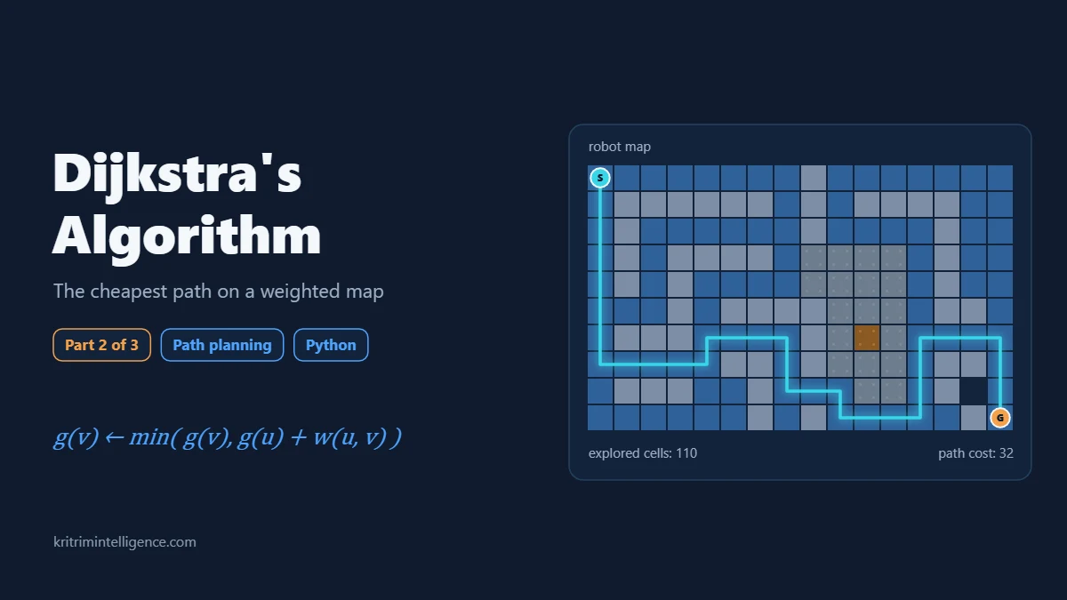
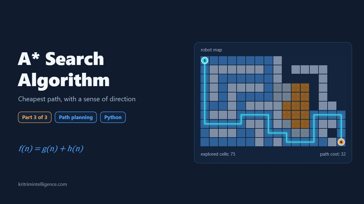
This is the last post in a three part series on path planning. Breadth first search found the route with the fewest steps but drove through mud. Dijkstra’s algorithm found the cheapest route but searched almost the whole map to be sure of it. A* finds the same cheapest route as Dijkstra while doing far less work. On our test map it settles 75 cells where Dijkstra settled 110.
Below we cover the idea behind A*, the conditions that keep it correct, how to choose a heuristic, and a Python version you can run on the same map as the earlier posts.
What this guide covers
- What is A* search?
- The score that drives A*: f = g + h
- Admissible and consistent heuristics
- How A* works, step by step
- Running time and memory
- Python example: A* on the robot grid map
- Choosing a heuristic: the trade off in numbers
- Watch A* drive a TurtleBot3 in ROS 2
- A* in robots today
- Frequently asked questions
- Closing thoughts
What is A* search?
A* is Dijkstra’s algorithm with a sense of direction. Dijkstra always expands the node that has been cheapest to reach so far. A* expands the node that looks cheapest overall: what it cost to get there, plus an estimate of what it will cost to finish the trip.
That estimate is called the heuristic. On a grid map, a simple heuristic is the distance to the goal ignoring walls. It costs almost nothing to compute, and it pulls the search toward the goal instead of letting it spread evenly in every direction.
The score that drives A*: f = g + h
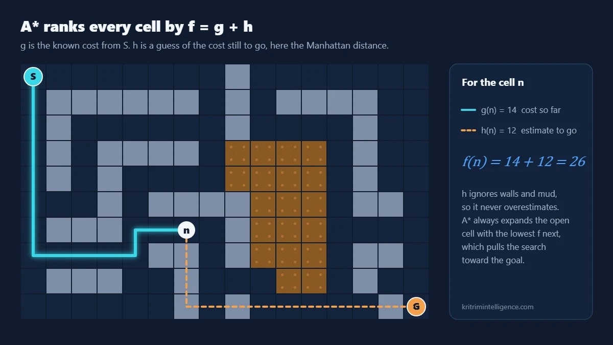
Every node n in A* carries three numbers:
- g(n) is the cost of the best path found so far from the start to n. This is the same value Dijkstra tracks.
- h(n) is the heuristic: an estimate of the cheapest cost from n to the goal.
- f(n) is their sum, the estimated cost of the best complete path that passes through n.
A* keeps its open nodes in a priority queue ordered by f and always expands the node with the lowest f. Everything else, the relaxing of edges, the parent links and the settled set, works just as it does in Dijkstra.
Two special cases make the idea clear. With h(n) equal to zero for every node, f is just g, and A* turns into Dijkstra. With a perfect heuristic that knows the true remaining cost, A* walks straight down the best path and expands almost nothing else. Every useful heuristic sits somewhere between those two.
Admissible and consistent heuristics
A* only promises the cheapest path if the heuristic follows a rule.
Admissible: never overestimate
A heuristic is admissible if it never guesses more than the true remaining cost. Writing h*(n) for the true cheapest cost from n to the goal:
The intuition is simple. If the estimate for the real best route were too high, that route could sit in the queue looking worse than it is while A* finishes with a more expensive path. An estimate that is too low can only make a route look better than it is, so A* checks it before it commits to an answer.
Consistent: no shortcuts through the estimate
A stronger rule, consistency, says the heuristic can never drop by more than the cost of a single move:
This is the triangle inequality applied to the estimate. A consistent heuristic is always admissible, and it brings a practical bonus: once a node is settled, its cost is final, exactly as in Dijkstra. That is why the code below can use the same settled set and skip old copies in the heap.
Manhattan distance on our grid
Our robot moves up, down, left or right, and every move costs at least 1. The Manhattan distance to the goal is
where r and c are the row and column. Any path to the goal needs at least that many moves, and each move costs at least 1, so Manhattan distance never overestimates. Each move changes it by exactly 1, so it is consistent too.
On maps where diagonal moves are allowed, Manhattan distance can overestimate. There the usual choices are the octile distance for 8 connected grids and straight line distance for free movement.
How A* works, step by step
- Set g(start) to 0 and push the start into the priority queue with priority h(start).
- Take the node n with the lowest f from the queue. Skip it if it is already settled.
- Mark n as settled. If n is the goal, follow the parent links back and stop.
- For each neighbour m of n, compute g(n) + w(n, m). If that beats the best known g(m), update g(m), set the parent of m to n and push m with priority g(m) + h(m).
- Repeat from step 2. An empty queue means there is no path.
Compared with Dijkstra, the only change is in step 4: the priority is g plus h instead of g alone.
Running time and memory
In the worst case, with a heuristic that tells the search nothing, A* expands as many nodes as Dijkstra and has the same running time, O((V + E) log V) with a binary heap.
In practice, everything depends on the heuristic. The better it predicts the true remaining cost, the fewer nodes A* touches. Hart, Nilsson and Raphael proved in 1968 that, with a consistent heuristic and no tie breaking luck, no other algorithm that uses the same heuristic and promises the cheapest path can expand fewer nodes than A*. In that sense, A* is as efficient as this kind of search can be.
Memory is the usual weak point. A* keeps every node it has seen in memory, and on large 3D maps that adds up. Variants such as iterative deepening A* trade extra time for much less memory.
Python example: A* on the robot grid map
Same map, same rules as before. S is the start, G is the goal, # is a wall, ~ is mud with a cost of 5 to enter, and . is open floor with a cost of 1.
The map and helper functions
# The map: S is the start, G is the goal, # is a wall,
# ~ is mud (slow to cross) and . is open floor.
GRID = [
    "S.......#.......",
    ".######.#.####..",
    ".#......#....#..",
    ".#.####.~~~~.#..",
    ".#.#....~~~~.#..",
    "...#.####~~~.##.",
    ".###....#~~~....",
    ".....##.#~~~.##.",
    ".###..#...~~.#..",
    "......#.#.....#G",
]
ROWS, COLS = len(GRID), len(GRID[0])
STEP_COST = {".": 1, "S": 1, "G": 1, "~": 5}   # cost to enter a cell


def find(symbol):
    for r, row in enumerate(GRID):
        if symbol in row:
            return (r, row.index(symbol))


def neighbours(cell):
    """Yield the open cells above, below, left and right of cell."""
    r, c = cell
    for dr, dc in ((-1, 0), (1, 0), (0, -1), (0, 1)):
        nr, nc = r + dr, c + dc
        if 0 <= nr < ROWS and 0 <= nc < COLS and GRID[nr][nc] != "#":
            yield (nr, nc)


def rebuild_path(parent, cell):
    """Walk the parent links back from the goal to the start."""
    path = []
    while cell is not None:
        path.append(cell)
        cell = parent[cell]
    return path[::-1]


def path_cost(path):
    return sum(STEP_COST[GRID[r][c]] for r, c in path[1:])


def show(path):
    on_path = set(path[1:-1])
    for r in range(ROWS):
        print("".join("*" if (r, c) in on_path else GRID[r][c] for c in range(COLS)))
The A* code
Compare this with the Dijkstra code from the previous post. The heap entries gain an f value at the front, and the push uses g plus the Manhattan distance. That is the whole difference.
import heapq


def manhattan(cell, goal):
    """Grid distance ignoring walls. Never more than the true cost,
    since every move costs at least 1."""
    return abs(cell[0] - goal[0]) + abs(cell[1] - goal[1])


def astar(start, goal):
    best = {start: 0}               # g: cheapest known cost from the start
    parent = {start: None}
    done = set()
    counter = 0
    frontier = [(manhattan(start, goal), counter, 0, start)]   # (f, tie, g, cell)
    expanded = 0
    while frontier:
        _, _, cost, cell = heapq.heappop(frontier)   # lowest f = g + h first
        if cell in done:
            continue
        done.add(cell)
        expanded += 1
        if cell == goal:
            return rebuild_path(parent, cell), cost, expanded
        for nxt in neighbours(cell):
            new_cost = cost + STEP_COST[GRID[nxt[0]][nxt[1]]]
            if new_cost < best.get(nxt, float("inf")):
                best[nxt] = new_cost
                parent[nxt] = cell
                counter += 1
                f = new_cost + manhattan(nxt, goal)
                heapq.heappush(frontier, (f, counter, new_cost, nxt))
    return None, float("inf"), expanded


start, goal = find("S"), find("G")
path, cost, expanded = astar(start, goal)
print(f"steps: {len(path) - 1}   cost: {cost}   cells expanded: {expanded}")
show(path)
Reading the result
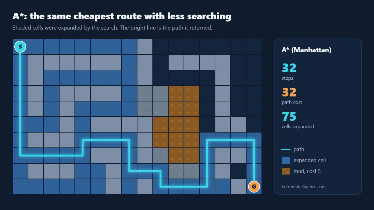
steps: 32   cost: 32   cells expanded: 75
S.......#.......
*######.#.####..
*#......#....#..
*#.####.~~~~.#..
*#.#....~~~~.#..
*..#.####~~~.##.
*###****#~~~****
*****##*#~~~*##*
.###..#***~~*#.*
......#.#****.#G
A* returns exactly the route Dijkstra found: 32 steps, a cost of 32 and no mud. It got there after settling 75 cells instead of 110, about a third less work. The cells it skipped are mostly in the top right corner, which lies far from the goal and only looked attractive to Dijkstra since it was cheap to reach.
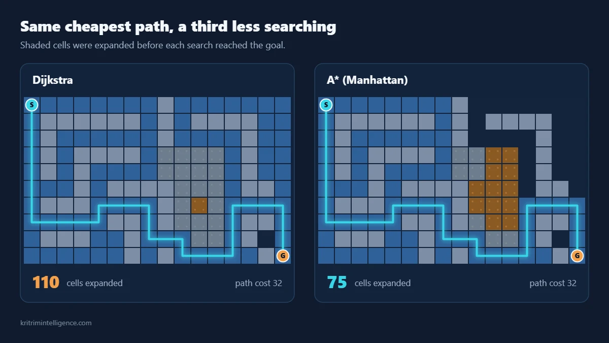
Here are all three algorithms side by side on the same map:
| Algorithm | Steps | Cost | Cells expanded |
|---|---|---|---|
| BFS | 24 | 48 | 111 |
| Dijkstra | 32 | 32 | 110 |
| A* (Manhattan) | 32 | 32 | 75 |
Choosing a heuristic: the trade off in numbers
The heuristic is the one part of A* you design yourself, so it is worth seeing what different choices do. Each row below is the same A* code on the same map with a different h:
| Heuristic | Steps | Cost | Cells expanded |
|---|---|---|---|
| h = 0 (Dijkstra) | 32 | 32 | 110 |
| Straight line distance | 32 | 32 | 83 |
| Manhattan distance | 32 | 32 | 75 |
| 2 × Manhattan | 32 | 32 | 46 |
| 5 × Manhattan | 36 | 36 | 43 |
Straight line distance is admissible here, but it is a looser estimate than Manhattan distance on a grid where the robot cannot move diagonally, so it saves less work. Manhattan distance is the tightest of the safe choices.
The last two rows multiply the heuristic by a weight. This is called weighted A*. The heuristic is no longer admissible, so the guarantee of the cheapest path is gone. In return the search becomes far greedier. With a weight of 2 it still happened to find the best path on this map while settling only 46 cells. With a weight of 5 it settled 43 cells but returned a path costing 36, about 12 percent worse. There is a useful bound here: with weight w, the path found never costs more than w times the cheapest one. Many real planners use a small weight on purpose, when a fast good path matters more than a slow perfect one.
Watch A* drive a TurtleBot3 in ROS 2
A 16 by 10 grid is good for learning. Here is the same algorithm on a real robot software stack. The video shows my A* planner running on a TurtleBot3 in a Gazebo simulation with ROS 2, viewed in RViz. The map the robot works on has 298 by 211 cells, about 63,000 in total.
Each time I set a goal in RViz, the planner runs A* on the occupancy grid, the green line appears, and the robot follows it. For the first goal, A* returned a path of 86 waypoints in 0.047 seconds. For a goal on the far side of the building it took 0.070 seconds for 83 waypoints. That speed is what lets a robot replan on the fly when something blocks its way.
A* in robots today
A* is rarely used in its textbook form on a real robot, but it is the core of many planners that are:
- Grid planners in ROS. The Nav2 stack in ROS 2 ships A* based global planners, and the older navfn planner offers A* as an option next to Dijkstra.
- Hybrid A*. Cars cannot turn on the spot, so Hybrid A* searches over position and heading and joins cells with drivable arcs. Stanford used it in the DARPA Urban Challenge, and the Smac planner in Nav2 includes it.
- Any angle planning. Theta* lets the path cut straight across open space instead of following grid edges, which gives shorter and smoother routes.
- Replanning. D* Lite reuses the work of earlier searches when the map changes, which suits robots that discover obstacles as they drive.
Frequently asked questions
What is the A* search algorithm in simple terms?
A* is a path finding algorithm that always expands the node with the lowest estimated total cost, f = g + h, where g is the cost from the start and h is an estimate of the cost to the goal. With a heuristic that never overestimates, it finds the cheapest path while exploring fewer nodes than Dijkstra.
What is the difference between A* and Dijkstra?
Dijkstra orders nodes by the cost from the start alone, so it searches evenly in every direction. A* adds a heuristic estimate of the remaining cost, which pulls the search toward the goal. Both find the cheapest path, but A* usually expands far fewer nodes.
What makes a heuristic admissible?
A heuristic is admissible if it never overestimates the true cheapest cost from a node to the goal. Manhattan distance on a 4 connected grid where every move costs at least 1 is a common example.
Is A* always optimal?
A* returns the cheapest path when its heuristic is admissible. If the heuristic overestimates, as in weighted A*, it can return a more expensive path in exchange for a faster search.
Which heuristic should I use for grid path planning?
Use Manhattan distance on 4 connected grids, octile distance on 8 connected grids and straight line distance when movement is free in any direction. Scale each by the lowest cost of a single move so the estimate stays admissible.
Closing thoughts
Across this series, one map has told the whole story. BFS counted steps and paid for it in mud. Dijkstra counted cost and found the cheap route, but looked almost everywhere to be sure. A* kept Dijkstra’s guarantee and added one line of distance math, and the search went straight for the goal.
That pattern, a cost for what you know plus an honest guess for what you do not, shows up all over robotics. Learn it on a 16 by 10 grid and you will recognise it inside much larger planners.
Which variant of A* runs on your robots? I would like to hear what has worked for you.
References
- P. E. Hart, N. J. Nilsson and B. Raphael, A formal basis for the heuristic determination of minimum cost paths, IEEE Transactions on Systems Science and Cybernetics 4(2), 100 to 107, 1968.
- I. Pohl, Heuristic search viewed as path finding in a graph, Artificial Intelligence 1(3), 1970.
- D. Dolgov, S. Thrun, M. Montemerlo and J. Diebel, Path planning for autonomous vehicles in unknown semi structured environments, International Journal of Robotics Research 29(5), 2010.
- S. Koenig and M. Likhachev, D* Lite, AAAI, 2002.
- A. Nash, K. Daniel, S. Koenig and A. Felner, Theta*: any angle path planning on grids, AAAI, 2007.
- Nav2 Smac Planner documentation: https://docs.nav2.org/configuration/packages/configuring-smac-planner.html
- S. J. Russell and P. Norvig, Artificial Intelligence: A Modern Approach, 4th edition, Pearson, 2020.