Markov Decision Process (MDP) Explained: Theory, Math and Python Code

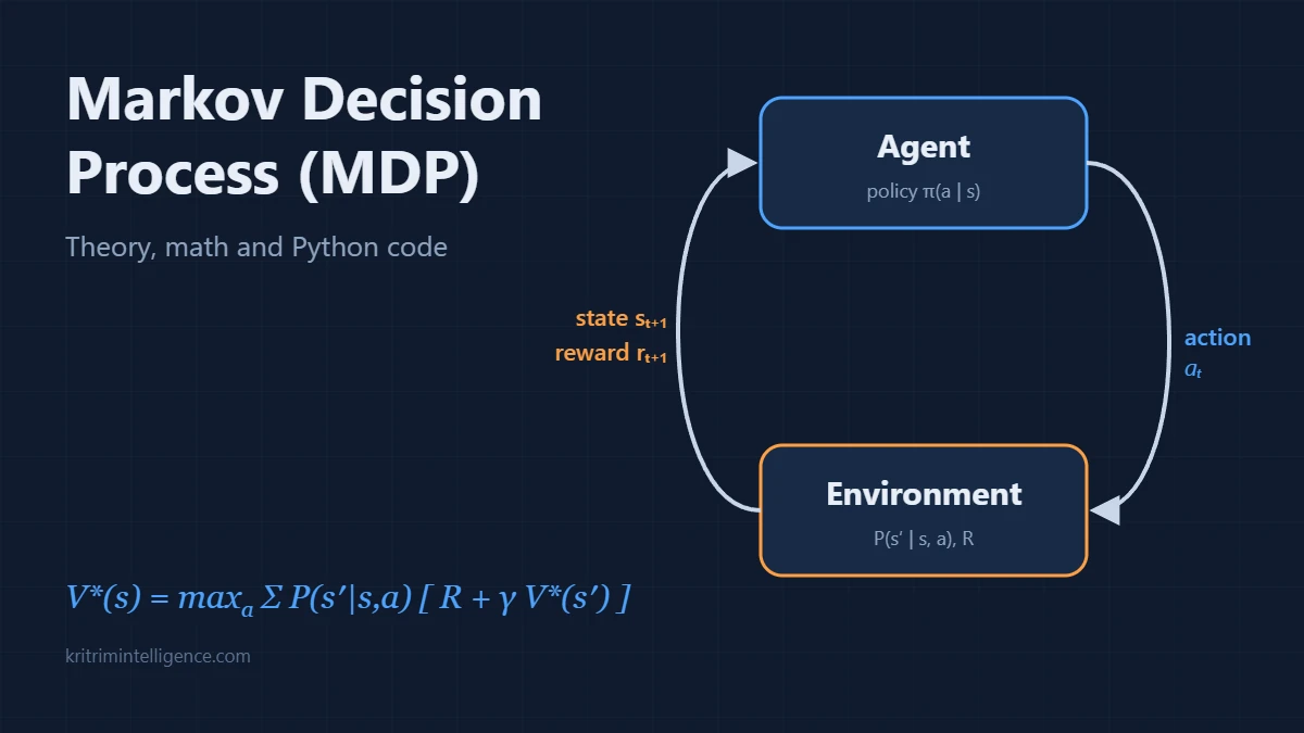
A Markov decision process (MDP) is the mathematical model behind almost every decision making problem in reinforcement learning. A robot choosing where to drive, a game agent picking its next move, a thermostat deciding when to heat: each one can be written as an MDP. Once a problem is in this form, we have clean tools to find the best possible behavior.

This guide builds the idea from the ground up. We start with plain language, add the formal notation step by step, derive the Bellman equations, and then solve a small grid world in Python with value iteration and policy iteration. Every number shown in the example comes from running the code below.

What is a Markov decision process?

A Markov decision process is a framework for sequential decision making under uncertainty. An agent observes the state of its world, takes an action, receives a reward, and lands in a new state. The new state is partly decided by the agent’s action and partly by chance. This loop repeats over and over.

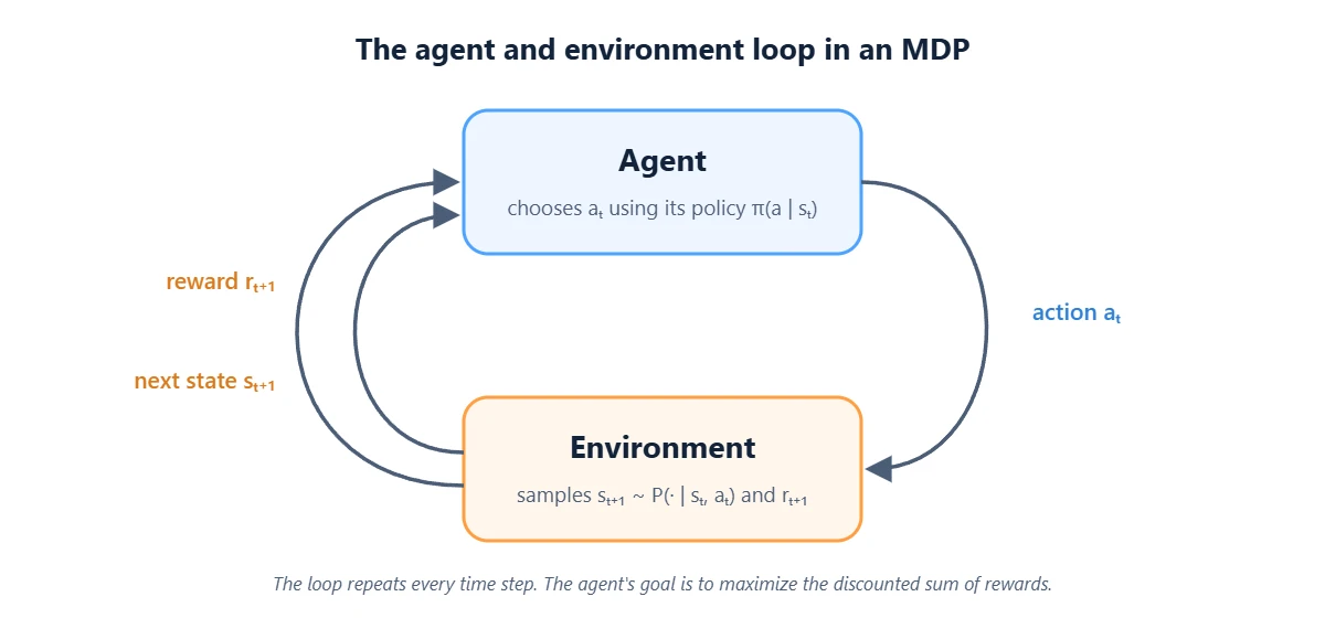
Formally, an MDP is a tuple of five parts:

• 𝒮 is the set of states the world can be in.
• 𝒜 is the set of actions the agent can take.
• P is the transition function: the probability of moving from one state to another after an action.
• R is the reward function: the number the agent receives after each step.
• γ (gamma) is the discount factor, a number between 0 and 1 that sets how much future rewards count.

The goal is to find a policy, a rule for picking actions, that collects as much reward as possible over time.

The Markov property

The word “Markov” comes from the Russian mathematician Andrey Markov. It refers to one assumption: the future depends only on the present state and action, not on the full history of how we got there.

In notation, with Sₜ for the state and Aₜ for the action at time t:

The left side looks only at the current state and action. The right side looks at everything that ever happened. The Markov property says they are equal. The current state already carries all the information you need to predict what comes next.

This is less restrictive than it sounds. If history matters, you can often fold the relevant history into the state. A chess position, for example, does not record every past move, but it contains everything needed to choose the next one. For a moving robot, adding velocity to the state alongside position usually restores the Markov property.

The five parts of an MDP in detail

States and actions

States describe the situation. In a grid world, a state is a cell. For a robot arm, it might be the joint angles and the position of the object. Actions are the choices available, such as up, down, left and right, or a set of motor commands. Here we focus on finite MDPs, where both sets are finite.

The transition function

The transition function gives the probability of each possible next state:

The probabilities over all next states add up to 1. This is where uncertainty lives. A robot that commands “move forward” might slip and end up somewhere else. In our grid world later, the intended move succeeds 80% of the time and the agent slips sideways the other 20%.

The reward function

The reward function tells the agent how good each step was:

Rewards are the only way we tell the agent what we want. Reaching a goal might give +1, every step might carry a small cost, and falling into a hole might end the episode with a penalty. Design the reward carefully: the agent will optimize exactly what you reward, not what you meant.

The discount factor and the return

The agent cares about the total reward it will collect from now on, called the return. Future rewards are multiplied by γ once for every step of delay:

With γ = 0.9, a reward one step away counts 0.9, two steps away 0.81, ten steps away about 0.35. A discount factor below 1 does three useful jobs: it keeps the infinite sum finite, it encodes a preference for sooner rewards, and it makes the math converge. Values close to 1 make the agent patient and far sighted. Values close to 0 make it greedy and short sighted.

Policies and value functions

Policies

A policy π tells the agent what to do in every state. A stochastic policy gives a probability for each action, and a deterministic policy picks one action per state:

State value and action value

To compare policies, we measure how much return each one earns. The state value function gives the expected return when starting in state s and following π:

The action value function, often called the Q function, gives the expected return when we take action a first and follow π afterwards:

The two are linked. The value of a state is the average action value under the policy:

The Bellman equations

Richard Bellman noticed in the 1950s that the value of a state can be written in terms of the values of the states that follow it. This recursive view is the heart of almost every MDP algorithm.

Bellman expectation equation

For a fixed policy π, the value of a state equals the expected immediate reward plus the discounted value of where you land next:

For a finite MDP this is a system of linear equations, one per state. Writing the policy’s transition matrix as P^π and its expected rewards as R^π, it has a closed form solution:

Solving it tells you exactly how good a given policy is. This step is called policy evaluation. For large state spaces we use the iterative version instead of the matrix inverse.

Bellman optimality equation

The optimal value function V* is the best value achievable from each state by any policy. Instead of averaging over the policy’s actions, it takes the best action:

The same idea in Q form:

Once you know Q*, the optimal policy simply picks the best action in each state:

Every finite MDP with γ < 1 has at least one optimal deterministic policy. That is a reassuring result: we never need randomness to act optimally when the model is fully known.

Solving an MDP: value iteration and policy iteration

When we know P and R, two classic dynamic programming algorithms find the optimal policy.

Value iteration

Value iteration turns the Bellman optimality equation into an update rule and applies it again and again:

1. Start with V(s) = 0 for every state.
2. Sweep over all states and apply the update above.
3. Stop when the largest change in any state during a sweep is smaller than a tiny threshold θ.
4. Read off the policy by picking the action with the highest value in each state.

Why does this converge? Call the update T. It is a contraction in the max norm:

Each sweep shrinks the distance to the true optimal values by at least a factor of γ. With γ = 0.9, the error falls by 10% or more on every sweep, so the values settle quickly and always reach the same answer no matter where you start.

Policy iteration

Policy iteration, introduced by Ronald Howard in 1960, alternates between two steps:

1. Policy evaluation: compute V^π for the current policy using the Bellman expectation equation.
2. Policy improvement: in each state, switch to the action with the highest Q value under V^π.

Repeat until the policy stops changing. Each round produces a policy at least as good as the last, and since a finite MDP has a finite number of deterministic policies, the process must end at an optimal one. Policy iteration usually needs very few rounds, though each round costs more as it includes a full evaluation.

Python example: solving a grid world MDP

Let us put all of this into code. Our world is a 4 × 4 grid:

• The agent can move up, down, left or right.
• Moves succeed with probability 0.8. With probability 0.1 each, the agent slips to one side instead.
• Walking into the wall or the edge leaves the agent where it is.
• The goal in the top right corner gives a reward of 1 and ends the episode.
• The pit directly below the goal ends the episode with a reward of −1.
• The discount factor is γ = 0.9.

The code uses only the Python standard library, so you can run it anywhere.

Step 1: define the states, actions, transitions and rewards

The function transitions returns P(s′, r | s, a) as a list of (probability, next state, reward) triples. This is the whole MDP in a few lines.

# 1. The MDP: a 4 x 4 grid world
ROWS, COLS = 4, 4
WALL = (1, 1)
GOAL = (0, 3)
PIT = (1, 3)
TERMINALS = {GOAL: 1.0, PIT: -1.0}   # reward for entering each terminal cell
ACTIONS = ["up", "down", "left", "right"]
MOVES = {"up": (-1, 0), "down": (1, 0), "left": (0, -1), "right": (0, 1)}
SLIPS = {"up": ["left", "right"], "down": ["left", "right"],
         "left": ["up", "down"], "right": ["up", "down"]}
GAMMA = 0.9

STATES = [(r, c) for r in range(ROWS) for c in range(COLS) if (r, c) != WALL]


def move(state, action):
    """Where the agent lands if it moves in `action`. Walls and edges block it."""
    dr, dc = MOVES[action]
    r, c = state[0] + dr, state[1] + dc
    if 0 <= r < ROWS and 0 <= c < COLS and (r, c) != WALL:
        return (r, c)
    return state


def transitions(state, action):
    """P(s', r | s, a) as a list of (probability, next_state, reward)."""
    if state in TERMINALS:
        return [(1.0, state, 0.0)]
    outcomes = [(0.8, action)] + [(0.1, slip) for slip in SLIPS[action]]
    result = []
    for prob, actual in outcomes:
        nxt = move(state, actual)
        result.append((prob, nxt, TERMINALS.get(nxt, 0.0)))
    return result

Step 2: value iteration in Python

The q_value function is the bracketed sum from the Bellman equation. Value iteration sweeps over the states, keeps the best action value, and stops when nothing changes by more than θ.

# 2. Value iteration
def q_value(V, s, a):
    """Expected return of taking action a in state s, then following V."""
    return sum(p * (r + GAMMA * V[s2]) for p, s2, r in transitions(s, a))


def value_iteration(theta=1e-6):
    V = {s: 0.0 for s in STATES}
    sweeps = 0
    while True:
        delta = 0.0
        for s in STATES:
            if s in TERMINALS:
                continue
            best = max(q_value(V, s, a) for a in ACTIONS)
            delta = max(delta, abs(best - V[s]))
            V[s] = best
        sweeps += 1
        if delta < theta:
            return V, sweeps


def greedy_policy(V):
    return {s: max(ACTIONS, key=lambda a: q_value(V, s, a))
            for s in STATES if s not in TERMINALS}

Step 3: policy iteration in Python

Policy iteration starts with a policy that always goes up, evaluates it, then improves it state by state until no change helps.

# 3. Policy iteration
def evaluate_policy(policy, V, theta=1e-6):
    while True:
        delta = 0.0
        for s in policy:
            v = q_value(V, s, policy[s])
            delta = max(delta, abs(v - V[s]))
            V[s] = v
        if delta < theta:
            return V


def policy_iteration():
    policy = {s: "up" for s in STATES if s not in TERMINALS}
    V = {s: 0.0 for s in STATES}
    rounds = 0
    while True:
        rounds += 1
        V = evaluate_policy(policy, V)
        stable = True
        for s in policy:
            best = max(ACTIONS, key=lambda a: q_value(V, s, a))
            if q_value(V, s, best) > q_value(V, s, policy[s]) + 1e-9:
                policy[s] = best
                stable = False
        if stable:
            return policy, V, rounds

Step 4: run it and print the results

# 4. Show the results
ARROWS = {"up": "↑", "down": "↓", "left": "←", "right": "→"}


def show(V, policy):
    for r in range(ROWS):
        values, arrows = [], []
        for c in range(COLS):
            s = (r, c)
            if s == WALL:
                values.append(" wall")
                arrows.append("■")
            elif s in TERMINALS:
                values.append(" goal" if s == GOAL else "  pit")
                arrows.append("G" if s == GOAL else "P")
            else:
                values.append(f"{V[s]:5.2f}")
                arrows.append(ARROWS[policy[s]])
        print("  ".join(values), "   ", " ".join(arrows))


if __name__ == "__main__":
    V, sweeps = value_iteration()
    print(f"Value iteration converged after {sweeps} sweeps\n")
    show(V, greedy_policy(V))
    pi, V2, rounds = policy_iteration()
    print(f"\nPolicy iteration converged after {rounds} rounds")
    print("Same policy as value iteration:", pi == greedy_policy(V))

Running the script prints:

Value iteration converged after 18 sweeps

 0.72   0.83   0.94   goal     → → → G
 0.63   wall   0.64    pit     ↑ ■ ↑ P
 0.54   0.47   0.53   0.37     ↑ ← ↑ ↓
 0.47   0.42   0.46   0.40     ↑ ↑ ↑ ←

Policy iteration converged after 4 rounds
Same policy as value iteration: True

Reading the results

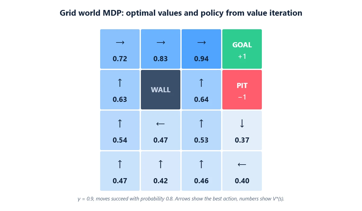
Value iteration converged after 18 sweeps and policy iteration after 4 rounds, and both found the same policy. Look at what the agent learned:

• Values grow toward the goal. The cell next to the goal is worth 0.94, and the bottom left corner is worth 0.47. Every step of distance costs a factor of γ, plus some risk of slipping.
• The agent steps away from danger. In the cell directly below the pit, moving up would land in the pit 80% of the time, and that action is worth −0.72. The policy moves down instead, where no slip can reach the pit.
• It takes the long way around. From the third row, second column, the shortest path to the goal passes right beside the pit. The policy goes left and climbs the left column around the wall instead. A few extra steps cost less than the chance of a −1.
• Risk is priced in. The cell to the left of the pit is worth only 0.64, far less than the 0.94 of the cell above it, as a sideways slip from there can drop the agent into the pit.

You can check one value by hand. Number rows and columns from 0, starting at the top left. From cell (0, 2), just left of the goal, the best action is right:

The 0.8 term is the successful move into the goal. The two 0.1 terms are slips: one bumps the top edge and stays put, the other drops to the cell below, worth 0.635. The result matches the 0.94 printed by the code.

Try changing the slip probability or γ and run it again. With γ = 0.99 the agent becomes more patient. Raise the slip chance to 0.4 and watch it take even wider detours around the pit.

How MDPs connect to reinforcement learning

Value iteration and policy iteration need the full model: every transition probability and every reward. In most real problems we do not have that. A robot does not come with a table of how likely each slip is.

Reinforcement learning solves the same MDP without knowing P and R in advance. The agent learns from experience instead. Q learning, for instance, nudges its estimate toward the Bellman optimality target after every real step:

Here α is a small learning rate, and the bracket is the gap between the Bellman target and the old estimate. Deep reinforcement learning replaces the table with a neural network so the same idea scales to images and huge state spaces. Methods like imitation learning and inverse reinforcement learning sit on top of the MDP framework too: they assume an MDP and learn the policy or the reward from demonstrations.

If you want to practice next, the FrozenLake environment in Gymnasium is a slippery grid world very close to the one above, and you can solve it with the same code after reading its transition table.

Variations and limits of MDPs

• Partially observable MDPs (POMDPs). The agent cannot see the full state, only noisy observations. A robot with a single camera often faces this. The agent then reasons about a belief, a probability distribution over states.
• Continuous states and actions. Robot joint angles and motor torques are continuous. Tables no longer work, so we use function approximation or control methods such as LQR.
• Average reward MDPs. For tasks that never end, some formulations maximize the average reward per step instead of a discounted sum.
• The curse of dimensionality. The number of states grows exponentially with the number of variables. Exact dynamic programming is only practical for small problems, which is the main reason sampled and approximate methods exist.

Frequently asked questions

Closing thoughts

Markov decision processes give a precise language for decisions under uncertainty: states, actions, transition probabilities, rewards and a discount factor. The Bellman equations turn that language into something we can compute, and value iteration and policy iteration solve it exactly for small problems. Everything in modern reinforcement learning, from Q learning to the systems that train robots and game agents, builds on these same ideas.

Copy the code, change the grid, add more pits or a step cost, and watch how the policy adapts. It is the fastest way to build a feel for how MDPs work. If you have questions, reach out through the contact page.

References

1. Bellman, R. (1957). Dynamic Programming. Princeton University Press.
2. Howard, R. A. (1960). Dynamic Programming and Markov Processes. MIT Press.
3. Puterman, M. L. (1994). Markov Decision Processes: Discrete Stochastic Dynamic Programming. Wiley.
4. Sutton, R. S., and Barto, A. G. (2018). Reinforcement Learning: An Introduction, second edition. MIT Press.
5. Russell, S., and Norvig, P. (2020). Artificial Intelligence: A Modern Approach, fourth edition. Pearson.
6. Watkins, C. J. C. H., and Dayan, P. (1992). Q learning. Machine Learning, 8, 279 to 292.
7. Farama Foundation. Gymnasium FrozenLake environment documentation.