In the first post of this series, breadth first search found the route with the fewest steps across a small robot map. It drove the robot straight through a patch of mud, for a trip that cost 48 when a cheaper route existed. BFS counts steps. It has no idea that some steps are harder than others.
Dijkstra’s algorithm fixes exactly that. It is the classic answer to the question robots, GPS units and network routers ask all day long: what is the cheapest way from here to there, when different moves have different costs? Edsger Dijkstra designed it in about twenty minutes at a café in Amsterdam in 1956, and seventy years later it is still in daily use.
This guide covers how the algorithm works, why it is correct, what it costs to run, and a Python version tested on the same map as the BFS post.
What is Dijkstra’s algorithm?
Dijkstra’s algorithm finds the cheapest path from one start node to every other node in a graph whose edges have costs that are zero or positive. If you only care about one goal, you can stop as soon as that goal is settled.
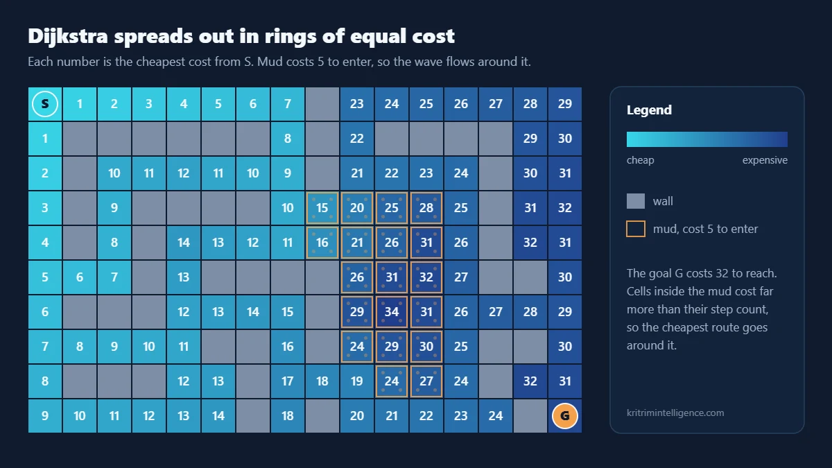
The cost of an edge can mean anything that adds up along a route: distance in metres, time in seconds, battery used, or a penalty for driving close to a wall. On our grid map, entering an open cell costs 1 and entering a mud cell costs 5.
Where BFS spreads out in rings of equal step count, Dijkstra spreads out in rings of equal cost. Cheap ground is covered quickly. Expensive ground holds the wave back, so the search flows around it when there is an easier way.
How Dijkstra works, step by step
The algorithm keeps the same three pieces of bookkeeping as BFS, with one important upgrade.
A best known cost for every node
For each node v, Dijkstra stores g(v), the cheapest cost found so far to reach v from the start. The start gets 0. Every other node starts at infinity, meaning no route is known yet.
A priority queue instead of a plain queue
BFS takes nodes in the order they were found. Dijkstra takes the node with the lowest g first, wherever it sits in the queue. A priority queue, usually a binary heap, does this efficiently: adding a node and removing the cheapest one each take time proportional to log n.
Relaxing edges
When Dijkstra takes a node u from the queue, it looks at each neighbour v and asks a simple question: is going through u cheaper than the best route to v I know so far? If it is, it updates the cost and the parent link. This check is called relaxing the edge:
Here w(u, v) is the cost of the move from u to v.
Settled nodes
Once a node comes out of the priority queue, its cost is final. Dijkstra marks it as settled and never changes it again. The search ends when the goal is settled, or when the queue is empty, which means the goal cannot be reached.
The full loop:
- Set g(start) to 0 and put the start in the priority queue.
- Take the node u with the lowest g from the queue. Skip it if it is already settled.
- Mark u as settled. If u is the goal, follow the parent links back and stop.
- For each neighbour v of u, relax the edge. If g(v) improved, record u as the parent of v and add v to the queue with its new cost.
- Repeat from step 2.
Why Dijkstra finds the cheapest path
The key claim is that when a node is taken from the queue, its cost is already the true cheapest cost. Here is the argument in plain words.
Suppose Dijkstra is about to settle node u with cost g(u), but some cheaper route to u exists. That cheaper route starts inside the settled region, so at some point it must leave it, through some node x that is still in the queue. The part of the route up to x already costs at least g(x), and g(x) is at least g(u), since u was picked as the cheapest node in the queue. The rest of the route, from x to u, cannot cost less than zero. So the whole route costs at least g(u), and it is not cheaper after all.
The last step depends on edge costs never being negative. With a negative edge, a route could look expensive halfway and then become cheap at the end, and a settled node could turn out to be wrong. For graphs with negative costs you need the Bellman Ford algorithm instead. Robot cost maps are never negative, so this limit rarely matters in practice.
Running time and memory
With a binary heap, every node is settled once and every edge can push one new entry into the heap. Each heap operation costs O(log V), which gives
On a grid with four neighbours per cell, E is about 4V, so this is O(V log V). Memory is O(V) for the costs, the parent links and the heap.
There is a faster theoretical bound using a Fibonacci heap, O(E + V log V), but its large constant factors mean the plain binary heap almost always wins in real code. On very large maps, engineers speed Dijkstra up in other ways: stopping at the goal, searching from both ends at once, or precomputing shortcuts, which is how online map services answer route queries across whole continents in milliseconds.
Python example: Dijkstra on the robot grid map
We use the same map and helper functions as the BFS post. S is the start, G is the goal, # is a wall, ~ is mud with a cost of 5 to enter, and . is open floor with a cost of 1.
The map and helper functions
# The map: S is the start, G is the goal, # is a wall,
# ~ is mud (slow to cross) and . is open floor.
GRID = [
    "S.......#.......",
    ".######.#.####..",
    ".#......#....#..",
    ".#.####.~~~~.#..",
    ".#.#....~~~~.#..",
    "...#.####~~~.##.",
    ".###....#~~~....",
    ".....##.#~~~.##.",
    ".###..#...~~.#..",
    "......#.#.....#G",
]
ROWS, COLS = len(GRID), len(GRID[0])
STEP_COST = {".": 1, "S": 1, "G": 1, "~": 5}   # cost to enter a cell


def find(symbol):
    for r, row in enumerate(GRID):
        if symbol in row:
            return (r, row.index(symbol))


def neighbours(cell):
    """Yield the open cells above, below, left and right of cell."""
    r, c = cell
    for dr, dc in ((-1, 0), (1, 0), (0, -1), (0, 1)):
        nr, nc = r + dr, c + dc
        if 0 <= nr < ROWS and 0 <= nc < COLS and GRID[nr][nc] != "#":
            yield (nr, nc)


def rebuild_path(parent, cell):
    """Walk the parent links back from the goal to the start."""
    path = []
    while cell is not None:
        path.append(cell)
        cell = parent[cell]
    return path[::-1]


def path_cost(path):
    return sum(STEP_COST[GRID[r][c]] for r, c in path[1:])


def show(path):
    on_path = set(path[1:-1])
    for r in range(ROWS):
        print("".join("*" if (r, c) in on_path else GRID[r][c] for c in range(COLS)))
The Dijkstra code
Python’s heapq module gives us a binary heap. Each entry is a tuple of cost, a counter and the cell. The heap orders by cost, and the counter breaks ties in insertion order, so the result is the same on every run.
Python’s heap has no way to lower the priority of an entry already inside it. The usual trick, used here, is to push a new entry with the lower cost and skip any old, more expensive copy when it comes out later. This is often called lazy deletion.
import heapq


def dijkstra(start, goal):
    best = {start: 0}               # cheapest known cost to reach each cell
    parent = {start: None}
    done = set()
    counter = 0                     # breaks ties in the same order every run
    frontier = [(0, counter, start)]
    expanded = 0
    while frontier:
        cost, _, cell = heapq.heappop(frontier)   # cheapest cell first
        if cell in done:
            continue                # an older, more expensive copy: skip it
        done.add(cell)
        expanded += 1
        if cell == goal:
            return rebuild_path(parent, cell), cost, expanded
        for nxt in neighbours(cell):
            new_cost = cost + STEP_COST[GRID[nxt[0]][nxt[1]]]
            if new_cost < best.get(nxt, float("inf")):
                best[nxt] = new_cost
                parent[nxt] = cell
                counter += 1
                heapq.heappush(frontier, (new_cost, counter, nxt))
    return None, float("inf"), expanded


start, goal = find("S"), find("G")
path, cost, expanded = dijkstra(start, goal)
print(f"steps: {len(path) - 1}   cost: {cost}   cells expanded: {expanded}")
show(path)
Reading the result
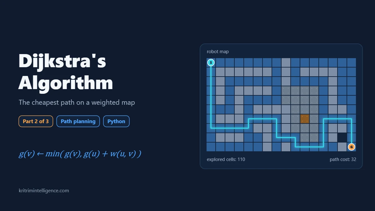
steps: 32   cost: 32   cells expanded: 110
S.......#.......
*######.#.####..
*#......#....#..
*#.####.~~~~.#..
*#.#....~~~~.#..
*..#.####~~~.##.
*###****#~~~****
*****##*#~~~*##*
.###..#***~~*#.*
......#.#****.#G
Dijkstra takes a completely different route from BFS. It heads down the left side, threads through the gap under the mud, climbs past the right edge of the mud and then drops down to the goal. The path is 32 steps long, eight more than the BFS path, and it does not touch a single mud cell. Its cost is 32, against 48 for BFS. That is a third less effort for the robot, and on a real machine it means less battery, less wheel slip and a lower chance of getting stuck.
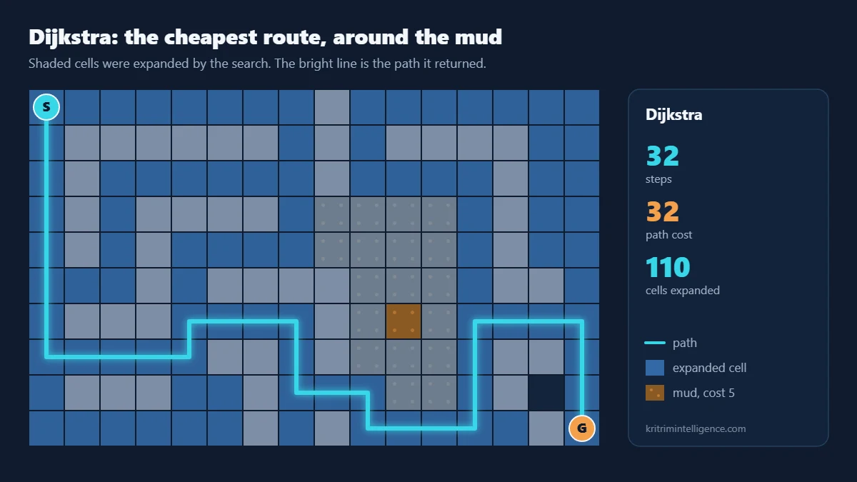
There is a price. To be sure it had the cheapest route, Dijkstra settled 110 of the 112 open cells, including many in the top right corner that lead nowhere useful. The algorithm has no sense of where the goal is. It grows outward evenly in cost, so it spends as much effort behind the robot as in front of it.
Here is how the two algorithms compare on the same map:
| Algorithm | Steps | Cost | Cells expanded |
|---|---|---|---|
| BFS | 24 | 48 | 111 |
| Dijkstra | 32 | 32 | 110 |
Where Dijkstra is used
- Grid and graph planners for mobile robots. The navfn global planner in ROS runs Dijkstra by default on a costmap that marks walls and the safety margin around them.
- Road maps and GPS. Route planning on road networks is built on Dijkstra, with extra speedups for very large maps.
- Network routing. The OSPF protocol that routes traffic inside large networks computes shortest paths with Dijkstra.
- A base for other algorithms. Uniform cost search in AI textbooks is Dijkstra with an early stop at the goal, and A* is Dijkstra plus a heuristic.
From Dijkstra to A*
Dijkstra gives the cheapest path every time, but it searches blindly in all directions. On a 16 by 10 grid that costs nothing. On a building map with millions of cells, planning has to happen many times per second, and wasted effort becomes a real problem.
The fix is to give the search a hint about which way the goal lies. If we add an estimate of the remaining cost to each node’s priority, cells that point toward the goal come out of the queue first, and cells behind the robot are often never looked at. That idea is A* search, and it is the subject of the last post in this series.
Frequently asked questions
What is Dijkstra’s algorithm used for?
Dijkstra’s algorithm finds the cheapest path in a graph where each edge has a cost that is zero or positive. It is used in robot path planning, GPS route planners, network routing protocols such as OSPF and as the base of A* search.
What is the difference between BFS and Dijkstra?
BFS takes nodes in the order they were found and finds the path with the fewest steps. Dijkstra takes the node with the lowest total cost first using a priority queue, so it finds the cheapest path when moves have different costs. With equal costs, both give paths of the same length.
Why does Dijkstra not work with negative edge weights?
Dijkstra treats a node’s cost as final once it leaves the priority queue. A negative edge found later could make that node cheaper, which breaks the guarantee. For graphs with negative costs, use the Bellman Ford algorithm.
What is the running time of Dijkstra’s algorithm?
With a binary heap, Dijkstra runs in O((V + E) log V) time, where V is the number of nodes and E is the number of edges. With a Fibonacci heap the bound is O(E + V log V).
Is Dijkstra the same as A*?
A* is Dijkstra with a heuristic added. Dijkstra orders nodes by the cost so far, g. A* orders them by g plus an estimate of the remaining cost, h. With h equal to zero, A* behaves exactly like Dijkstra.
Closing thoughts
Dijkstra’s algorithm is the point where path planning starts to care about the ground under the robot. One change, swapping a plain queue for a priority queue ordered by cost, turns BFS into a planner that steers around mud, ramps and crowded aisles on its own.
Its weakness is focus. It checks almost the whole map to guarantee one path. In the final post of this series we keep the same map and add one line of distance math to the priority, and A* finds the very same cheapest path while settling far fewer cells.
What costs do you put on your robot’s map? I would like to hear how you set them up.
References
- E. W. Dijkstra, A note on two problems in connexion with graphs, Numerische Mathematik 1, 269 to 271, 1959.
- T. H. Cormen, C. E. Leiserson, R. L. Rivest and C. Stein, Introduction to Algorithms, 4th edition, MIT Press, 2022. Chapter on single source shortest paths.
- S. M. LaValle, Planning Algorithms, Cambridge University Press, 2006. Free online: https://lavalle.pl/planning/
- M. L. Fredman and R. E. Tarjan, Fibonacci heaps and their uses in improved network optimization algorithms, Journal of the ACM 34(3), 1987.
- ROS navfn package: http://wiki.ros.org/navfn
- Python documentation, heapq: https://docs.python.org/3/library/heapq.html