The "Faster Than Dijkstra" Algorithm Is Slower Than Dijkstra. The Benchmarks Prove It.
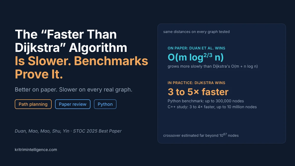
Headlines said a 2025 algorithm beat Dijkstra. On paper it does. In Python and C++ benchmarks, Dijkstra was 3 to 5 times faster. Here is why both are true.
For more than sixty years, Dijkstra's algorithm has been the answer to one of the most common questions in computing: what is the cheapest way from here to everywhere else? It runs inside internet routers, map apps and the global planners of robots, including the grid planner in our Dijkstra's algorithm explainer. For about forty years, many computer scientists assumed that on general directed graphs, nothing could beat it by more than a constant factor.
In 2025 a team led by Ran Duan at Tsinghua University proved otherwise. Their paper, "Breaking the Sorting Barrier for Directed Single-Source Shortest Paths", won a Best Paper Award at STOC 2025, one of the top conferences in theoretical computer science. Soon articles, videos and posts everywhere were calling it the algorithm that is faster than Dijkstra.
It is not. Not on any graph you will ever run. What the paper proves is narrower: its running time grows more slowly than Dijkstra's as sparse directed graphs get larger, with fixed overhead left out of the count. That is a real result, and a hard one. But when we implemented the algorithm in Python and raced it against Dijkstra, Dijkstra won at every size, by 3 to 5 times. A careful C++ study on road networks of up to 10 million nodes found the same thing.
This post explains what the "sorting barrier" is, how the new algorithm gets around it, why "faster in theory" and "faster" are two different claims, and what the paper did achieve. We checked our version against Dijkstra on 1,600 random graphs and on the same robot grid map from our Dijkstra post.
What this guide covers
The paper at a glance
| Title | Breaking the Sorting Barrier for Directed Single-Source Shortest Paths |
| Authors | Ran Duan, Jiayi Mao, Xiao Mao, Xinkai Shu, Longhui Yin |
| Institutions | Tsinghua University, Stanford University |
| Venue | STOC 2025, Best Paper Award |
| Link | arXiv:2504.17033 |
| Running time | O(m log^(2/3) n), against O(m + n log n) for Dijkstra with a Fibonacci heap |
| Follow up | O(m √(log n · log log n)) on sparse graphs, February 2026 (arXiv:2602.07868) |
Here n is the number of nodes and m is the number of edges. On a sparse graph, such as a road network or a robot's grid map, m is roughly a small multiple of n.
Why Dijkstra hits a "sorting barrier"
Dijkstra's algorithm works outward from the start. At every step it picks the unsettled node with the smallest known distance, settles it, and updates its neighbours. A priority queue makes "pick the smallest" fast, and that is where the n log n part of its running time comes from.
Look at the order in which Dijkstra settles nodes. It is exactly the nodes sorted by distance from the start. In other words, Dijkstra sorts as a side effect, and sorting n numbers by comparing them needs about n log n comparisons. Any algorithm that settles nodes one by one in distance order is stuck with that cost. This is the sorting barrier.
There is an important twist. In 2024, Bernhard Haeupler, Richard Hladík, Václav Rozhoň, Robert Tarjan and Jakub Tětek proved that Dijkstra, with the right kind of heap, is "universally optimal" if you want the nodes in sorted order. That paper won a best paper award at FOCS 2024. So Dijkstra cannot be beaten at its own game. The only way to go faster is to stop playing it: find all the distances without ever putting the nodes in order.
That is what Duan and his coauthors did.
How the new algorithm works
The algorithm mixes two classic ideas. Dijkstra is fast per node but keeps a sorted frontier. Bellman-Ford needs no sorting at all, but it is slow, since it relaxes every edge over and over. The new algorithm uses a little of each, inside a recursion.
Idea 1: shrink the frontier with a few Bellman-Ford rounds
The frontier is the set of nodes that have a distance estimate but are not settled yet. The more nodes it holds, the more sorting Dijkstra has to do. The first routine, which the paper calls FindPivots, shrinks it.
From the current frontier, it runs only k rounds of Bellman-Ford relaxation, where k is tiny: roughly the cube root of log n. After those rounds, any node whose shortest path is fewer than k edges away from the frontier is already correct. For the rest, the routine looks at the shortest path trees that grew from each frontier node. Most nodes hang off a few large trees. The roots of those large trees become pivots, and only the pivots stay in the frontier. The paper shows the frontier shrinks by about a factor of k this way.
Idea 2: recurse on distance bands
The main routine, BMSSP (bounded multi source shortest path), takes a distance bound B and a set of sources, and finds every node closer than B that is reached through those sources. It does not process the frontier one node at a time. It pulls out a whole batch of the closest pivots, hands them to a smaller recursive call with a tighter bound, and repeats. At the bottom of the recursion, a tiny Dijkstra run settles a handful of nodes.
Idea 3: only partly sort
The batches come from a special data structure that keeps the frontier only partly sorted. It can hand out "the next M smallest" as a group, without fixing the order inside the group. With about log^(1/3) n levels of recursion and carefully chosen batch sizes, the total cost comes to O(m log^(2/3) n) instead of the n log n sorting cost.
The paper chooses k = log^(1/3) n and t = log^(2/3) n, where t sets how fast batch sizes grow from one level of recursion to the next.
How big is the gain on paper?
For sparse graphs, Dijkstra's cost per edge grows like log n, and the new algorithm's like log^(2/3) n. Here is what those factors look like, using base 2 logs and ignoring constant factors, which a big O bound leaves out:
| Nodes n | Dijkstra (log n) | Duan et al. 2025 (log^(2/3) n) | Duan et al. 2026 (√(log n · log log n)) |
|---|---|---|---|
| 1 million | 19.9 | 7.4 | 9.3 |
| 1 billion | 29.9 | 9.6 | 12.1 |
| 2^64 | 64.0 | 16.0 | 19.6 |
| 2^1000 | 1000 | 100 | 99.8 |
Two things stand out. The gap over Dijkstra grows slowly, about 3 times at a billion nodes. And the 2026 bound, though better in the long run, only overtakes the 2025 bound on paper for graphs with roughly 2^991 nodes, far more than there are atoms in the universe. Bounds like these are about what is possible, not about which code to ship.
A Python implementation, checked against Dijkstra
We wrote a teaching version of the algorithm in Python, following the paper's three routines: FindPivots, BaseCase and BMSSP. One simplification: the paper's partly sorted data structure is replaced by an ordinary heap. That keeps the code short and the answers correct, but it means this version does not reach the paper's running time bound. Treat it as a way to see the algorithm work, not as a fast library.
One detail matters. The paper assumes no two paths have exactly the same length. Our first test used whole number weights, which create many ties, and the results were wrong on 120 of 400 graphs. Adding a tiny random amount to every edge weight, a standard way to break ties, fixed it completely.
Save this as bmssp.py:
"""Duan, Mao, Mao, Shu and Yin (2025): shortest paths without fully sorting the frontier.

A teaching version of the recursive algorithm (BMSSP) from "Breaking the Sorting
Barrier for Directed Single-Source Shortest Paths". It follows the paper's three
routines: FindPivots, BaseCase and BMSSP. The partial sorting structure D is
simplified to a heap, so this version shows the idea and gives correct answers,
but it does not reach the paper's running time bound.
"""
import heapq
import math

INF = float("inf")


class Frontier:
    """Simplified version of the paper's data structure D (Lemma 3.3)."""

    def __init__(self, M, B):
        self.M, self.B = M, B
        self.best = {}                    # vertex -> smallest value seen
        self.heap = []

    def insert(self, v, value):
        if value < self.best.get(v, INF):
            self.best[v] = value
            heapq.heappush(self.heap, (value, v))

    batch_prepend = insert                # the paper's BatchPrepend, simplified

    def _clean(self):
        while self.heap and self.best.get(self.heap[0][1]) != self.heap[0][0]:
            heapq.heappop(self.heap)

    def empty(self):
        self._clean()
        return not self.heap

    def pull(self):
        """Take up to M vertices with the smallest values.
        Return them and a bound that separates them from everything left."""
        S = []
        while len(S) < self.M and not self.empty():
            _, v = heapq.heappop(self.heap)
            del self.best[v]
            S.append(v)
        self._clean()
        bound = self.heap[0][0] if self.heap else self.B
        return bound, S


class SSSP:
    def __init__(self, graph, source):
        self.g = graph                    # graph[u] = list of (v, weight)
        n = len(graph)
        logn = max(math.log2(n), 2)
        self.k = max(1, int(logn ** (1 / 3)))
        self.t = max(1, int(logn ** (2 / 3)))
        self.d = [INF] * n
        self.parent = [None] * n
        self.d[source] = 0.0
        levels = math.ceil(logn / self.t)
        self.relaxations = 0
        self.bmssp(levels, INF, [source])

    def relax(self, u, v, w):
        """Shared relaxation step. Uses <= so equal paths are passed on, as in the paper."""
        self.relaxations += 1
        nd = self.d[u] + w
        if nd <= self.d[v]:
            if nd < self.d[v]:
                self.parent[v] = u
            self.d[v] = nd
            return nd
        return None

    # ---------------------------------------------------------------- Algorithm 1
    def find_pivots(self, B, S):
        """Run k rounds of Bellman-Ford from S. Keep as pivots only the sources
        whose shortest path trees reach at least k vertices."""
        W, layer = set(S), set(S)
        for _ in range(self.k):
            nxt = set()
            for u in layer:
                for v, w in self.g[u]:
                    nd = self.relax(u, v, w)
                    if nd is not None and nd < B:
                        nxt.add(v)
            W |= nxt
            layer = nxt
            if len(W) > self.k * len(S):
                return list(S), W         # frontier already small enough
        children = {u: [] for u in W}
        for v in W:
            p = self.parent[v]
            if p in children and v not in S:
                children[p].append(v)
        pivots = []
        for s in S:                       # size of the tree hanging off each source
            size, stack = 0, [s]
            while stack and size < self.k:
                size += 1
                stack.extend(children[stack.pop()])
            if size >= self.k:
                pivots.append(s)
        return pivots, W

    # ---------------------------------------------------------------- Algorithm 2
    def base_case(self, B, S):
        """A small Dijkstra run from one vertex, stopped after k + 1 vertices."""
        x = S[0]
        done, heap = [], [(self.d[x], x)]
        seen = set()
        while heap and len(done) < self.k + 1:
            du, u = heapq.heappop(heap)
            if u in seen or du != self.d[u]:
                continue
            seen.add(u)
            done.append(u)
            for v, w in self.g[u]:
                nd = self.relax(u, v, w)
                if nd is not None and nd < B:
                    heapq.heappush(heap, (nd, v))
        if len(done) <= self.k:
            return B, done
        Bp = max(self.d[v] for v in done)
        return Bp, [v for v in done if self.d[v] < Bp]

    # ---------------------------------------------------------------- Algorithm 3
    def bmssp(self, level, B, S):
        """Settle every vertex whose distance is below B and whose shortest path
        passes through S, working on a frontier of limited size."""
        if level == 0:
            return self.base_case(B, S)
        pivots, W = self.find_pivots(B, S)
        D = Frontier(2 ** ((level - 1) * self.t), B)
        for x in pivots:
            D.insert(x, self.d[x])
        Bp_i = min((self.d[x] for x in pivots), default=B)
        U = set()
        limit = self.k * 2 ** (level * self.t)
        while len(U) < limit and not D.empty():
            B_i, S_i = D.pull()
            Bp_i, U_i = self.bmssp(level - 1, B_i, S_i)
            U.update(U_i)
            K = []
            for u in U_i:
                for v, w in self.g[u]:
                    nd = self.relax(u, v, w)
                    if nd is None:
                        continue
                    if B_i <= nd < B:
                        D.insert(v, nd)
                    elif Bp_i <= nd < B_i:
                        K.append((v, nd))
            for x in S_i:
                if Bp_i <= self.d[x] < B_i:
                    K.append((x, self.d[x]))
            for v, val in K:
                D.batch_prepend(v, val)
        Bp = min(Bp_i, B)
        U.update(x for x in W if self.d[x] < Bp)
        return Bp, U
Testing it on the robot grid map
The demo below builds the same 16 by 10 grid from our Dijkstra post, where mud costs 5 and open floor costs 1, runs the new algorithm from the top left corner, and prints the route. Then it races both algorithms on random sparse graphs with three edges per node.
import heapq
import random
import time

from bmssp import SSSP

# ---------------------------------------------------------------- 1. the grid map from the Dijkstra post
GRID = [
    "S.......#.......",
    ".######.#.####..",
    ".#......#....#..",
    ".#.####.~~~~.#..",
    ".#.#....~~~~.#..",
    "...#.####~~~.##.",
    ".###....#~~~....",
    ".....##.#~~~.##.",
    ".###..#...~~.#..",
    "......#.#.....#G",
]
ROWS, COLS = len(GRID), len(GRID[0])
STEP_COST = {".": 1, "S": 1, "G": 1, "~": 5}
rng = random.Random(0)


def cell_id(r, c):
    return r * COLS + c


graph = [[] for _ in range(ROWS * COLS)]
for r in range(ROWS):
    for c in range(COLS):
        if GRID[r][c] == "#":
            continue
        for dr, dc in ((-1, 0), (1, 0), (0, -1), (0, 1)):
            nr, nc = r + dr, c + dc
            if 0 <= nr < ROWS and 0 <= nc < COLS and GRID[nr][nc] != "#":
                # The paper assumes no two paths have exactly the same length.
                # A tiny random amount on each edge breaks the ties.
                w = STEP_COST[GRID[nr][nc]] + rng.random() * 1e-9
                graph[cell_id(r, c)].append((cell_id(nr, nc), w))

start, goal = cell_id(0, 0), cell_id(ROWS - 1, COLS - 1)
result = SSSP(graph, start)

path, v = [], goal
while v is not None:
    path.append(v)
    v = result.parent[v]
on_path = set(path[1:-1])
print(f"cost to the goal: {result.d[goal]:.0f}   steps: {len(path) - 1}")
for r in range(ROWS):
    print("".join("*" if cell_id(r, c) in on_path else GRID[r][c] for c in range(COLS)))


# ---------------------------------------------------------------- 2. a race on random road style graphs
def dijkstra(graph, source):
    dist = [float("inf")] * len(graph)
    dist[source] = 0.0
    heap = [(0.0, source)]
    while heap:
        du, u = heapq.heappop(heap)
        if du > dist[u]:
            continue
        for v, w in graph[u]:
            if du + w < dist[v]:
                dist[v] = du + w
                heapq.heappush(heap, (dist[v], v))
    return dist


print("\n     nodes   same answer   Dijkstra   new algorithm")
for n in [10_000, 100_000, 300_000]:
    g = [[(rng.randrange(n), rng.random()) for _ in range(3)] for _ in range(n)]
    t0 = time.perf_counter()
    a = dijkstra(g, 0)
    t1 = time.perf_counter()
    b = SSSP(g, 0).d
    t2 = time.perf_counter()
    print(f"{n:>10,}   {str(a == b):>11}   {t1 - t0:>7.2f} s   {t2 - t1:>11.2f} s")
Running it prints:
cost to the goal: 32   steps: 32
S.......#.......
*######.#.####..
*#......#....#..
*#.####.~~~~.#..
*#.#....~~~~.#..
*..#.####~~~.##.
*###****#~~~****
*****##*#~~~*##*
.###..#***~~*#.*
......#.#****.#G

     nodes   same answer   Dijkstra   new algorithm
    10,000          True      0.01 s          0.05 s
   100,000          True      0.33 s          1.20 s
   300,000          True      1.27 s          4.44 s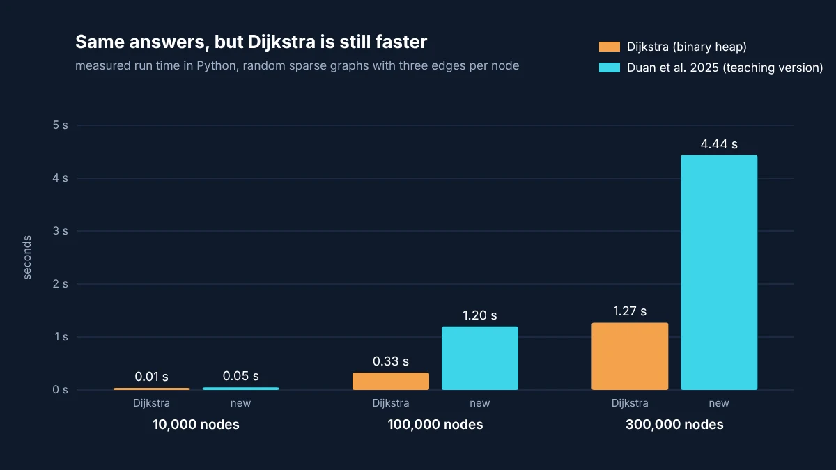
On the grid, the new algorithm finds the same route as Dijkstra in our earlier post: 32 steps, a cost of 32, and not a single mud cell. On random graphs of up to 300,000 nodes it agreed with Dijkstra on every distance. Beyond this demo, we tested it on 1,600 random graphs, including 1,000 with whole number weights and tie breaking, and it matched Dijkstra every time.
And Dijkstra was 3 to 5 times faster on every size. Our heap based simplification is part of that, but not all of it.
Is it faster in practice?
No. In November 2025, Lucas Castro, Thailsson Clementino and Rosiane de Freitas published a careful C++ implementation of the full algorithm, including its special data structure. They tested sparse random graphs, grids and US road networks with up to 10 million nodes. Dijkstra was 3 to 4 times faster in every case. They estimate the number of nodes would need to be far larger than 10^67 before the worst case version overtakes Dijkstra.
The reason is constant factors. Big O notation hides them, and this algorithm has large ones: several layers of recursion, Bellman-Ford rounds that relax the same edges more than once, and a more complex data structure. A binary heap is simple and very fast on real hardware. A log n factor of 20 is hard to beat when your own constant factor is bigger than that.
What this means for robots and path planning
If you are writing a robot planner, keep using Dijkstra or A*. On a grid map with a few hundred thousand cells, a well written Dijkstra finishes in milliseconds in a compiled language, and A* with a good heuristic does less work still, as our A* explainer showed on the same grid. Planners such as Nav2 in ROS 2 are built on these for good reason.
So why does this paper matter? Three reasons:
- It corrects the textbook. For decades, "Dijkstra is optimal" was close to accepted wisdom for this problem. That was only true for algorithms that sort.
- It opens a new direction. Within a year, the same team improved their own bound. Smaller constant factors may follow, and history shows that theory results sometimes become practical once people find simpler versions.
- The ideas are useful on their own. Shrinking a frontier with a few cheap relaxation rounds, and working in batches instead of strict order, are tricks that apply in parallel and GPU shortest path methods too.
Frequently asked questions
Is there an algorithm faster than Dijkstra?
Not in practice. In 2025, Duan, Mao, Mao, Shu and Yin proved a deterministic algorithm for sparse directed graphs whose running time, O(m log^(2/3) n), grows more slowly than Dijkstra's O(m + n log n). On every real graph tested so far, up to 10 million nodes, Dijkstra is 3 to 4 times faster, and one study estimates the crossover lies far beyond 10^67 nodes.
What is the sorting barrier in shortest paths?
Dijkstra settles nodes in order of distance from the start, which means it sorts them as a side effect. Sorting n items by comparison takes about n log n steps, so any algorithm that works this way cannot go faster. The new algorithm breaks the barrier by finding all the distances without putting the nodes in order.
How does the new shortest path algorithm work?
It combines Dijkstra and Bellman-Ford inside a recursion. A few rounds of Bellman-Ford shrink the frontier to a small set of pivot nodes, then the algorithm processes pivots in batches over shrinking distance bands, using a data structure that keeps the frontier only partly sorted.
Who discovered the sorting barrier algorithm?
Ran Duan, Jiayi Mao, Xiao Mao, Xinkai Shu and Longhui Yin, from Tsinghua University and Stanford University. Their paper won a Best Paper Award at STOC 2025, and the group published an improved version in February 2026.
Should I replace Dijkstra in my robot path planner?
No. The new algorithm is a theoretical breakthrough, but its constant factors are large. Benchmarks on grids and road networks found Dijkstra 3 to 4 times faster, and A* with a good heuristic is usually faster still for single goal robot planning.
Is the "faster than Dijkstra" claim true?
Only on paper. The paper proves a better running time bound, and that proof is correct and peer reviewed. Calling the algorithm faster than Dijkstra misleads, since Dijkstra finishes first on every real graph tested so far.
Closing thoughts
What stands out about this result is the way it got around the barrier. Nobody built a better sorting method. The authors noticed that the problem never asked for sorted output, and that Dijkstra was doing extra work by producing it anyway. Many hard limits in computing turn out to be limits of one approach, not of the problem itself.
So here is the honest summary. The proof is real, and the headline was not. "Faster than Dijkstra" holds only for graphs far larger than any computer could store. If you saw that claim and pictured a drop in replacement for Dijkstra, it does not exist yet.
If you run the code, try printing the frontier size before and after FindPivots on a large graph to watch it shrink. We would like to hear whether anyone finds a graph where it beats Dijkstra in Python.
References
- R. Duan, J. Mao, X. Mao, X. Shu and L. Yin, Breaking the Sorting Barrier for Directed Single-Source Shortest Paths, STOC 2025. arXiv:2504.17033
- R. Duan, X. Mao, X. Shu and L. Yin, A Faster Directed Single-Source Shortest Path Algorithm, 2026. arXiv:2602.07868
- L. Castro, T. Clementino and R. de Freitas, Implementation and Brief Experimental Analysis of the Duan et al. (2025) Algorithm for Single-Source Shortest Paths, 2025. arXiv:2511.03007
- B. Haeupler, R. Hladík, V. Rozhoň, R. Tarjan and J. Tětek, Universal Optimality of Dijkstra via Beyond-Worst-Case Heaps, FOCS 2024. arXiv:2311.11793
- E. W. Dijkstra, A note on two problems in connexion with graphs, Numerische Mathematik, 1959.