Diffusion Policy Explained: How Robots Learn Multimodal Actions, with Python Code

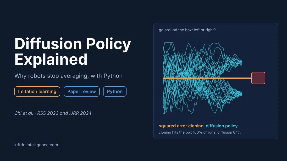
Picture a robot arm in front of a box, and a pile of demonstrations from people showing it how to get past. Half of them went around the left side. The other half went around the right. Both are good answers. Now train the simplest kind of imitation learning policy on that data, and watch what it does. It drives straight into the box.

That is not a bug in the code. It is what a policy trained with squared error is built to do: when the demonstrations disagree, it predicts their average, and the average of left and right is straight ahead. Diffusion Policy, published in 2023 by Cheng Chi, Shuran Song, Russ Tedrake and colleagues at Columbia, MIT and Toyota Research Institute, fixed this by borrowing the idea behind AI image generators. Instead of predicting one action, the robot starts from random noise and refines it, step by step, into an action that looks like one of the demonstrations.

Diffusion Policy is one of the papers in my imitation learning course this semester, and three years later its core idea sits inside many of the large robot models released in 2026. This post walks through the problem it solves, how it works, what the experiments showed, and a small Python example, written in plain NumPy, that you can run to watch a diffusion policy pick a side while ordinary cloning crashes. If imitation learning is new to you, start with my overview of imitation learning and the DAgger explainer.

The paper at a glance

Title	Diffusion Policy: Visuomotor Policy Learning via Action Diffusion
Authors	Cheng Chi, Zhenjia Xu, Siyuan Feng, Eric Cousineau, Yilun Du, Benjamin Burchfiel, Russ Tedrake, Shuran Song
Institutions	Columbia University, Toyota Research Institute, MIT
Venue	RSS 2023, extended version in IJRR 2024
Link	arXiv:2303.04137
Main idea	Generate robot actions the way image models generate pictures: start from noise and remove it step by step, guided by what the robot sees

Why plain behavior cloning averages

Behavior cloning treats robot control as supervised learning. You record what the robot saw and what the person did, then train a network to map one to the other. The usual training loss is squared error between the predicted action and the demonstrated one.

Squared error has a well known property: the single prediction that minimises it is the mean of the targets. That is fine when every demonstrator does roughly the same thing. It goes wrong when there are several good answers, which happens constantly in real tasks:

• Going around an obstacle on the left or the right.
• Grasping a mug by the handle or by the rim.
• Pushing a block from one side first or the other.

In each case the average of two good actions can be a bad one. Researchers call this a multimodal action distribution, where each separate good answer is a mode. Earlier work tried to fix it with mixtures of Gaussians (LSTM-GMM), energy based models (Implicit Behavioral Cloning, or IBC) and discretised actions (Behavior Transformers, or BET). Each helped, and each had trouble: mixtures need you to guess how many modes there are, and energy based models are hard to train.

How Diffusion Policy works

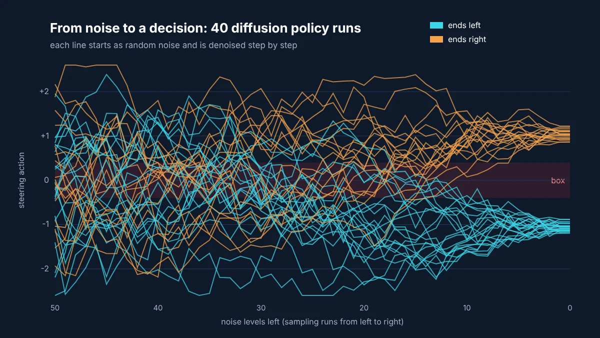
A diffusion model learns to reverse a noising process. During training you take a clean example, add a random amount of noise to it, and ask a network to predict the noise you added. At run time you start from pure noise and use the network to remove a little noise at a time until a clean sample appears. Image generators do this with pixels. Diffusion Policy does it with robot actions.

Training

For each training example:

1. Take a short sequence of demonstrated actions, along with the camera images and robot state the person saw at that moment.
2. Pick a random noise level k and add that much Gaussian noise to the actions.
3. Ask the network to predict the noise, given the noisy actions, the noise level and the observation.
4. Update the network with squared error between the predicted noise and the real noise.

The loss is still squared error, but it is applied to the noise, not to the action. That small change is what makes multimodal data safe. The network never has to commit to one average action. It only learns, at every noise level, which direction leads back toward the demonstrations.

Running the policy

At run time the robot:

1. Starts with a sequence of actions drawn from pure noise.
2. Runs the network K times. Each pass predicts the noise in the current guess and removes a bit of it, conditioned on the latest camera images.
3. Ends with a clean action sequence that looks like something a demonstrator would do.

The random starting point decides which mode the robot lands in. One run might start closer to "go left" and end there. Another starts closer to "go right". What it will not do is land halfway between, since the training data never pointed there.

The paper trains with 100 noise levels. On the real robots it uses a faster sampler called DDIM to cut that to roughly 10 to 16 steps at run time, which brought inference down to about 0.1 seconds on an NVIDIA RTX 3080.

Three design choices that made it work on robots

The diffusion part gets the attention, but three practical choices in the paper matter just as much.

1. Predict a sequence of actions, then replan. The policy predicts 16 future actions at once, runs the first 8, then looks again and predicts a fresh sequence. This is called receding horizon control. Predicting a whole sequence keeps the motion smooth and consistent, so the robot does not flip between left and right on every step. Replanning every 8 steps keeps it responsive when something moves.

2. Use the camera as a condition, not as part of the output. The images are encoded once and fed into every denoising step, through a technique called FiLM that scales and shifts the network's internal features. The network only has to generate actions, not images, which keeps it fast.

3. Command positions, not velocities. Most earlier methods output velocities. The authors found Diffusion Policy did consistently better with position targets, and they give three reasons: position commands show more clearly separated modes, which diffusion handles well; they build up less error over time; and they held up better when the authors added delay to the control loop.

The paper offers two network types. A 1D convolutional network is the recommended starting point and needs little tuning. A transformer version is better on tasks where actions change quickly and sharply, though it needs more care to train.

What the experiments showed

On simulation benchmarks (Robomimic, Push-T, multimodal Block Pushing and Franka Kitchen), Diffusion Policy improved average success by 46.9 percent over the best earlier methods. The real robot results were even clearer.

Real robot task	Diffusion Policy	Best earlier method
Push-T (push a T shaped block into place)	95% success	20% (LSTM-GMM), 0% (IBC)
Mug flipping	90% of 20 trials	LSTM-GMM never grasped the mug
Sauce pouring on pizza dough	79% success	0% (LSTM-GMM)
Sauce spreading	100% success	0% (LSTM-GMM)

On Push-T, human demonstrators scored an overlap of 0.84 with the target and Diffusion Policy scored 0.80, close to human level. The IJRR version added bimanual tasks with two arms: 55 percent on an egg beater task, and 75 percent on both mat unrolling and shirt folding.

The project page shows the multimodal behavior directly. On Push-T, LSTM-GMM tended to get stuck near the block, IBC ended episodes early, and BET switched between strategies in the middle of a run. Diffusion Policy picked one strategy per run and stuck with it.

A small Python example: averaging vs diffusion

Here is the box problem from the start of this post, in about 85 lines of NumPy with no deep learning library. 2,000 demonstrations steer left (around minus 1) or right (around plus 1), half each. Steering anywhere between minus 0.4 and 0.4 hits the box.

The first policy is behavior cloning with squared error, which reduces to the mean of the demos. The second is a tiny diffusion policy: a two layer network trained to predict noise across 50 noise levels, then sampled from pure noise.

import numpy as np

rng = np.random.default_rng(0)

# ------------------------------------------------------------ the demonstrations
# A box sits straight ahead. Half the operators steer left around it (-1),
# half steer right (+1). Steering between -0.4 and 0.4 hits the box.
N = 2000
demos = np.where(rng.random(N) < 0.5, -1.0, 1.0) + rng.normal(0, 0.1, N)


def hits_box(a):
    return np.abs(a) < 0.4


# ------------------------------------------------------------ 1. behavior cloning with squared error
# The single action that minimises squared error is the mean of the demos.
bc_action = demos.mean()

# ------------------------------------------------------------ 2. a tiny diffusion policy
T = 50                                         # number of noise levels
betas = np.linspace(1e-4, 0.2, T)
alphas = 1.0 - betas
alpha_bar = np.cumprod(alphas)


def features(x, t):
    """Network input: the noisy action and a few sine features of the noise level."""
    s = t[:, None] / T
    return np.hstack([x[:, None], np.sin(np.pi * s * [1, 2, 4]), np.cos(np.pi * s * [1, 2, 4])])


# A small two layer network, trained with plain numpy and Adam.
H = 64
params = {
    "W1": rng.normal(0, 0.5, (7, H)), "b1": np.zeros(H),
    "W2": rng.normal(0, 0.2, (H, H)), "b2": np.zeros(H),
    "W3": rng.normal(0, 0.2, (H, 1)), "b3": np.zeros(1),
}
adam = {k: [np.zeros_like(v), np.zeros_like(v)] for k, v in params.items()}


def predict_noise(x, t):
    f = features(x, t)
    h1 = np.tanh(f @ params["W1"] + params["b1"])
    h2 = np.tanh(h1 @ params["W2"] + params["b2"])
    return (h2 @ params["W3"] + params["b3"])[:, 0], (f, h1, h2)


for step in range(1, 15001):
    a0 = rng.choice(demos, 256)                # clean demo actions
    t = rng.integers(0, T, 256)                # a random noise level for each
    eps = rng.normal(size=256)                 # the noise we add
    xt = np.sqrt(alpha_bar[t]) * a0 + np.sqrt(1 - alpha_bar[t]) * eps
    pred, (f, h1, h2) = predict_noise(xt, t)
    g = 2 * (pred - eps)[:, None] / len(eps)   # gradient of mean squared error
    grads = {"W3": h2.T @ g, "b3": g.sum(0)}
    g2 = (g @ params["W3"].T) * (1 - h2 ** 2)
    grads.update({"W2": h1.T @ g2, "b2": g2.sum(0)})
    g1 = (g2 @ params["W2"].T) * (1 - h1 ** 2)
    grads.update({"W1": f.T @ g1, "b1": g1.sum(0)})
    for k in params:                           # Adam update
        m, v = adam[k]
        m[:] = 0.9 * m + 0.1 * grads[k]
        v[:] = 0.999 * v + 0.001 * grads[k] ** 2
        params[k] -= 3e-3 * (m / (1 - 0.9 ** step)) / (np.sqrt(v / (1 - 0.999 ** step)) + 1e-8)


def sample(n):
    """Start from pure noise and denoise step by step (DDPM sampling)."""
    x = rng.normal(size=n)
    for t in reversed(range(T)):
        eps_hat, _ = predict_noise(x, np.full(n, t))
        x = (x - betas[t] / np.sqrt(1 - alpha_bar[t]) * eps_hat) / np.sqrt(alphas[t])
        if t > 0:
            x += np.sqrt(betas[t]) * rng.normal(size=n)
    return x


actions = sample(1000)

print(f"behavior cloning (squared error): steers {bc_action:+.2f} every time, "
      f"hits the box {hits_box(np.array([bc_action])).mean():.0%} of the time")
print(f"diffusion policy, 1000 runs:      left {np.mean(actions < -0.4):.1%}   "
      f"right {np.mean(actions > 0.4):.1%}   hits the box {hits_box(actions).mean():.1%}")

Running it prints (training takes about 10 seconds on a laptop):

behavior cloning (squared error): steers -0.01 every time, hits the box 100% of the time
diffusion policy, 1000 runs:      left 48.1%   right 51.8%   hits the box 0.1%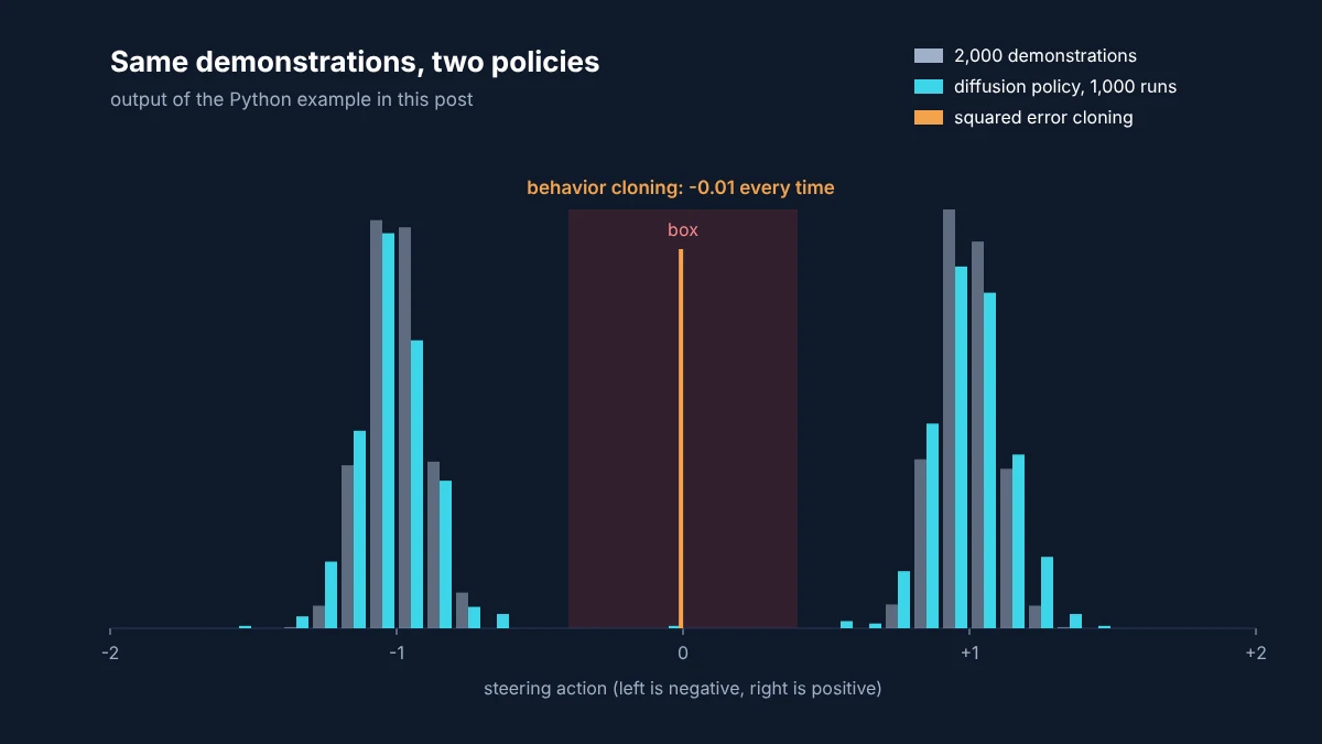

The squared error policy learned to steer at minus 0.01, straight ahead, and hits the box on every run. The diffusion policy split its 1,000 runs almost evenly between left and right, matching the demonstrations, and only 1 run in 1,000 landed in the box. Both policies saw exactly the same data. The difference is only in what they were trained to predict.

A few things to try with the code:

• Change the split so 80 percent of demos go left. The diffusion policy follows the new proportions.
• Reduce training to 6,000 steps. The policy still steers clear of the box, but the left and right split drifts away from even, a sign the network has not fully learned the weights of each mode.
• Reduce T to 10 noise levels. Sampling is five times faster. In my run, box hits rose from 0.1 to 0.4 percent, an early sign of where quality starts to drop.

Diffusion Policy in robots today

The paper changed what a default robot policy looks like. In 2026 its ideas show up almost everywhere:

• Large robot models generate actions this way. NVIDIA's GR00T N1.7 uses a 32 layer diffusion transformer for motor control, and Physical Intelligence's π0 family uses flow matching, a close relative of diffusion that reaches clean actions in fewer steps.
• Action chunks are standard. Predicting a short sequence and replanning, used both here and in ACT (Action Chunking with Transformers), is now the normal way to run a learned manipulation policy.
• Reinforcement learning on top. Methods like FlowDPG fine tune diffusion and flow policies with reinforcement learning after imitation, which I covered in Beyond Imitation.
• Still a strong baseline. In the REAL-I challenge at ICRA 2026, a small Diffusion Policy trained from scratch scored full marks on one task where large pretrained models did not.

The main costs are speed and data. Even with DDIM, a diffusion policy needs several network passes per decision, which is slow for very fast control loops. And like any imitation method, it can only reproduce behaviors that appear in the demonstrations.

Frequently asked questions

Closing thoughts

The lesson I take from Diffusion Policy is that the loss function decides what a policy can express. Squared error can only ever give one answer per situation, so it blends good answers into bad ones. Changing what the network predicts, from the action to the noise, let the same kind of network keep every good answer it was shown.

If you run the example, try making the two groups of demonstrations uneven, or move them closer together until they touch. I would like to hear at what point the diffusion policy stops telling them apart.

References

• C. Chi, Z. Xu, S. Feng, E. Cousineau, Y. Du, B. Burchfiel, R. Tedrake and S. Song, Diffusion Policy: Visuomotor Policy Learning via Action Diffusion, RSS 2023 and IJRR 2024. arXiv:2303.04137
• Diffusion Policy project page, Columbia University. diffusion-policy.cs.columbia.edu
• J. Ho, A. Jain and P. Abbeel, Denoising Diffusion Probabilistic Models, NeurIPS 2020. arXiv:2006.11239
• J. Song, C. Meng and S. Ermon, Denoising Diffusion Implicit Models, ICLR 2021. arXiv:2010.02502
• T. Z. Zhao, V. Kumar, S. Levine and C. Finn, Learning Fine-Grained Bimanual Manipulation with Low-Cost Hardware (ACT), RSS 2023. arXiv:2304.13705
• NVIDIA, Isaac GR00T N1.7: open reasoning VLA model for humanoid robots, 2026. Hugging Face blog